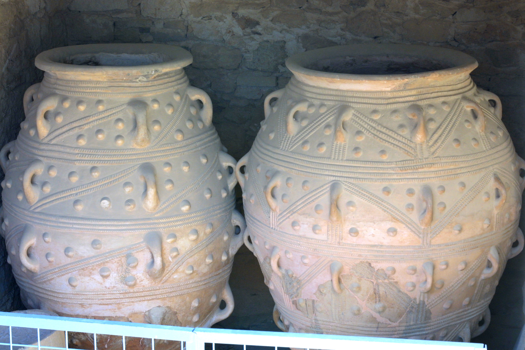
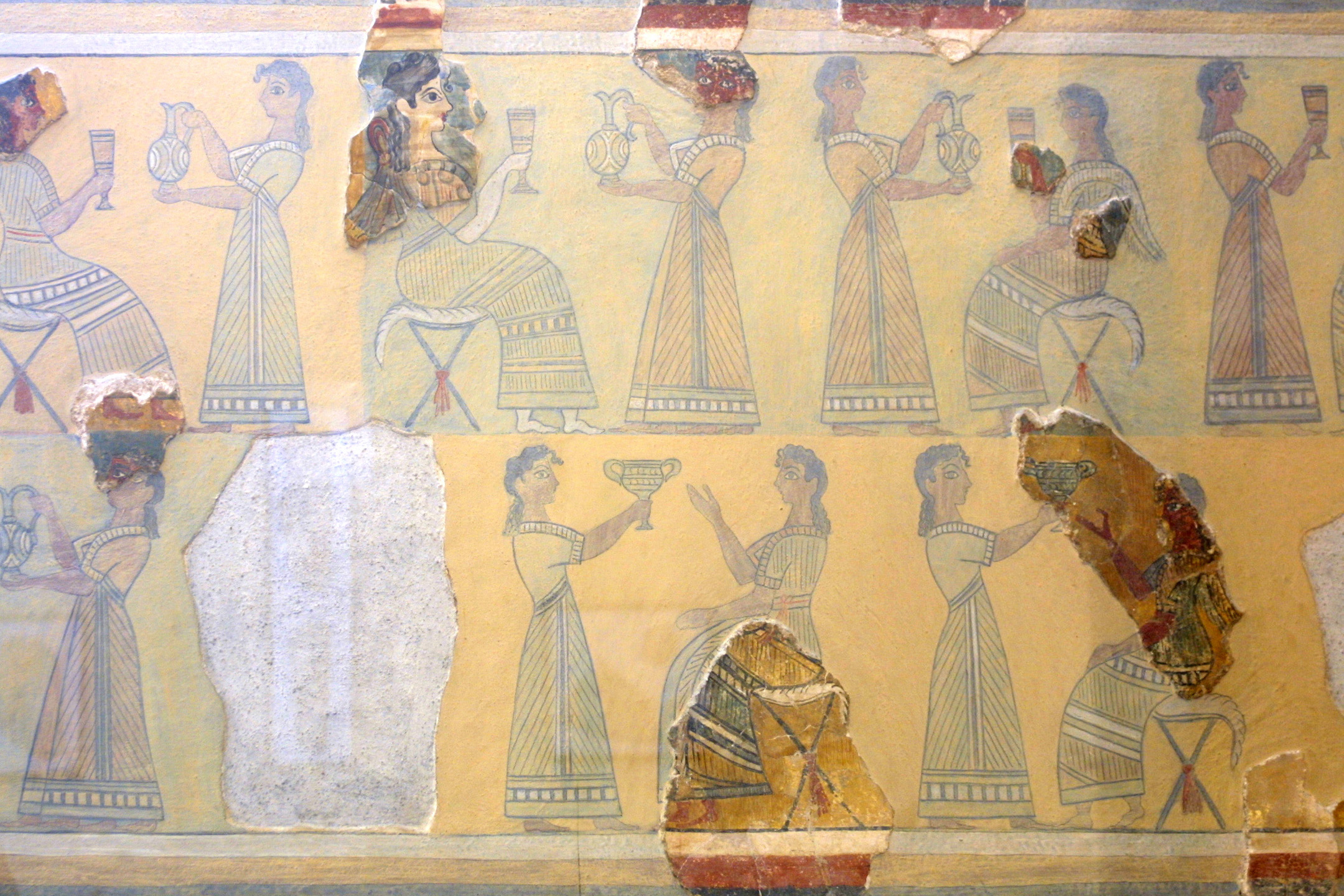
![]() Three positions of bull-leaping sports. Bulls were worshiped by Phoenicians and Canaanites in Palestine. |
![]() Water jars. Cretans carried water with these jars to the ritual baths. |
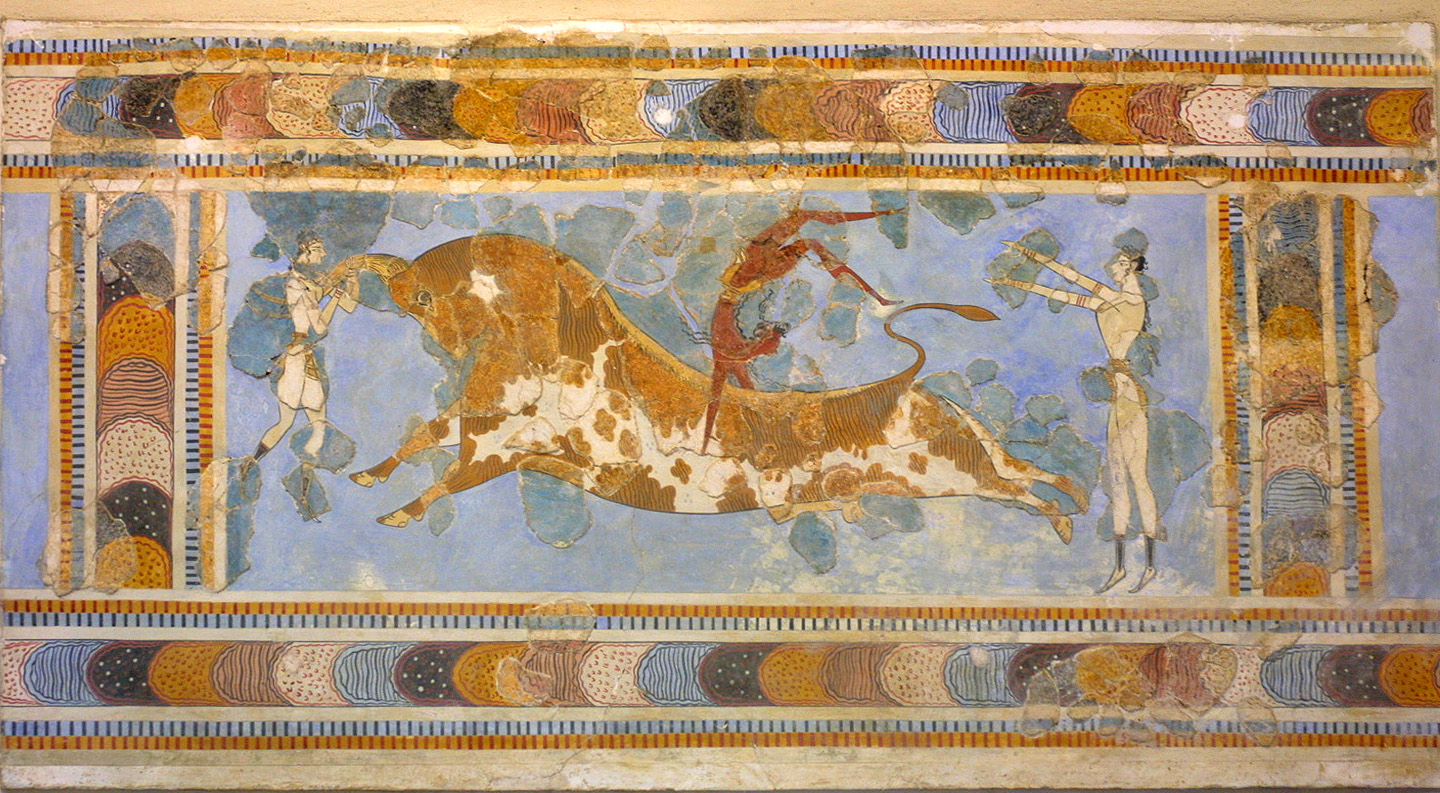
![]() Life in the Knossos Palace, a restored mural. |
![]() Linear B tablet (Omniglot) with syllabaries, partly deciphered, similar to hiragana). A precursor of alphabet. |
JAPAN |
Tatemoto and Ichimura
(1959) studied Japan's trade pattern and discovered another paradox. Japan
was a labor-abundant country, but exported capital-intensive goods and imported
labor- intensive goods. Japan's overall trade pattern was
inconsistent with HO. Explanation: They said that Japan's place in the world was somewhere between advanced and LDCs. 75% of exports went to LDCs.
Japan-LDC, consistent. |
East Germany |
Stolper and Roskamp (1961) applied Leontief's method to the trade pattern of East Germany. East Germany's exports were capital-intensive. About 3/4 of EG's trade was with the communist bloc, and EG was capital abundant relative to its trading partners. Thus, the EG case was consistent with the HO theory. |
| South Korea | Hong (1975) analyzed Korea's trade pattern (1966-72), which was consistent with the HO theory. |
| CANADA | Wahl (1961) studied Canada's trade pattern. Canadian exports were capital-intensive. Most of Canadian trade was with the US. The result was inconsistent with HO. |
| INDIA | Bharawaj (1962) studied India's trade pattern. India's
exports were labor-intensive. Consistent with HO theory. However, Indian trade with the US was not. Indian exports to the US were capital-intensive. |
Roughly half the countries tested show trade patterns consistent with the HO theory. In such cases, there must be some problems that offset the HO trade patterns. The HO theory generally explains the trade patterns during the post war periods, say 1960 - 2000. World trade patterns have become a lot more complex. Major changes: outsourcing which is sensitive to factor price differentials. US manufacturing firms outsource fragmented processes to low wage countries. |
| Leontief | Leontief himself suggested an explanation
for his own paradox. He argued that US workers may be more efficient than
foreign workers. Perhaps U.S. workers were three times as effective as
foreign workers. Note that this increased effectiveness of the American
workers was not due to a higher capital-labor ratio, because we assume
that countries have identical technologies and hence identical capital-
labor ratios. It means that the average American worker is three times as effective as he would be in the foreign country. Given the same K/L ratio, Leontief attributed the superior efficiency of American labor to superior economic organization and economic incentives in the U.S. However, Leontief found very few believers among economists. |
| Empirical evidence | Kreinin (1965) conducted a survey of engineers
and managers, and tried to test whether an average American worker is
three times as effective as a foreign worker. A realistic
difference in effectiveness between the representative
workers in the U.S. and those in the foreign countries were about 20-25%.
Obviously, this difference does not explain the Leontief Paradox.
When comparing trade patterns of a market economy and a command economy, this explanation may be important. Modern technology is available to Russians, but production in the former Soviet Union is still inefficient due to lack of incentives. |
| Evaluation | There might have been some difference in labor efficiency or productivity between the US and the rest of world in 1947. But this should have been relatively insiginficant. This was probably a bad theory. |
| Trefler (1993) resurrects Leontief's theory and has proved that when quality indices of factors are incorporated, US exported capital and imported labor services in 1947 (HOV Theorem). This still does not prove, however, that US exports had been more capital intensive than its imports that year. |
| If a commodity
is produced by a labor-intensive process in the labor-rich country and
also by the capital-intensive process in the capital-rich country, then
factor intensities are reversed in the production of that commodity.
Example: agriculture is labor-intensive in India but capital-intensive in US. If the US imports agricultural products, then an LP occurs in the US, because a capital abundant country is importing the capital-intensive product. If the US exports agricultural products, then an LP occurs in India, because a labor-abundant country, India, is importing the labor-intensive good. |
|
| LP is inevitable | In the presence of FIR, the HO theory cannot hold for both countries. That is, an LP always occurs in one of the countries. Thus, Jones (1956) and Robinson (1956) argued that FIR could have been responsible for the LP in the US. |
| Empirical relevance | The question is whether FIR
is common in the real world. Minhas (1963) investigated
24 industries for which comparable data were available for 19 countries.
He found FIRs only in 5 countries. Leontief (1964) reviewed Minhas's book and pointed out that only 17 out of 210 possible reversals did occur for the relevant range of factor prices. Moroney (1967) concluded that FIR has much less empirical importance, albeit theoretically interesting. |
| Agriculture | Remark: FIR plays
an important role only if the trade volume of the industries with reversed
factor intensities is large. While there has not been much empirical evidence about the possibility of factor intensity reversals, FIR is real. It may be important when comparing trade patterns between developing and developed economies (e.g. China vs. US). In most developed economies agriculture's share of GDP is less than 1%.(UK = .7%, US = 1.2%, world = 6.1%). Thus, empirical FIR is not important. |
| Leontief may have oversimplified the production functions and failed to recognize the endowments of natural resources. With three factors of production, the HO model does not predict much. This is because the notion of abundance and intensity must be redefined. | |
| "Factor intensities" are difficult to define in higher dimensions. | It is possible to have K1/L1 > K2/L2 and K1/N1 < K2/N2. |
| Jaroslav Vanek's Argument (1963) | Suppose the US is poor in natural resources. Assume that the import-competing industry uses capital and natural resources in fixed proportions, i.e., K and L are perfect complements in production. Then apply the HO theory. The US imports natural resource-intensive products, but it appears that the US is importing the capital- intensive goods. |
| Evaluation | Empirical studies have shown that the natural resource content in typical US imports is greater than that in US exports. But it is difficult to believe that US is poor in natural resources. Vanek's explanation is not empirically convincing. |
| Factor Abundance is meaningful | In a world of many factors (K, L, N, .... Z), factor
abundance can be ranked: K/K* > N/N*> ...> L/L*. In this case, we can say that the HC is (most) abundant in capital, and least abundant in labor. |
| Heckscher-Ohlin-Vanek Theorem | A country
exports its abundant factors through trade in goods. Let a = Y/(Y + Y*) be the home country's share of world income. Then the HC is abundant in capital, if
Of course, this definition can be extended to any other factors. According to this definition, it is possible for a country to be abundant in more than one factors. The HOV Theorem states that if trade is balanced a country exports its abundant factors through trade in goods. China's labor share = 1.4 billion/7 billion = 0.2 China's income share = 1/7. 0.2 > 1/7. China will export labor services through international trade. The purpose of trade is to exports the abundant factor. |
| Remark | 1. If factor prices are equalized, the definition of factor abundance makes sense, since income is the sum of factor incomes.
K/K* > Y/Y* if and only if K/K* > L/L*.
2. Trade theory is supposed to predict the patterns of output trade. As the number of outputs increases, it becomes exceedingly difficult to predict the patterns of output trade. Thus, HOV was not even a result that economists were looking for. 3. Nevertheless, HOV theorem predicts the indirect trade of factors through output trade. If HOV prediction is not materialized in the real world, it is an indication that there is a serious distortion in the economy. In this sense, HOV Theorem does provide a guide to trade policy; a trade policy should not encourage exports of scarce resources and imports of abundant resources. |
| Travis (1964) argued that tariff may have been responsible for the LP. However, tariffs tend to reduce trade volume, but not reverse commodity trade pattern. In other words, an import tariff cannot induce a country to export goods that intensively use its scarce factor. It would only reduce the volume of goods which it would export in the absence of a tariff. | |
Baldwin (1971) showed that this indeed was the case. Without tariff, the capital-labor ratio of imports would have fallen by 5%, which is not sufficient to resolve the LP.
|
|
| Remark | Tariffs and transport costs tend to reduce the volume of trade, but not reverse the pattern of trade. |
| A capital abundant country need not export the capital-intensive good if her tastes are strongly biased toward capital-intensive goods. Thus, LP can be explained if the US had a strong consumption bias toward the capital-intensive goods. | |
| Example of demand bias | In 1819 Francois-Louis Cailler established one of the first chocolate factories in Switzerland. Cailler Swiss Chocolate is the oldest brand of Swiss chocolate still in existence, and Switzerland leads the world in per capita annual chocolate consumption, 22.5 pounds per person! (Swiss Chocholate). Per capita consumption of chocolates is less than 5 pounds in the United States. Per capita consumption of seafood in Japan is 60 kg per year while that of the US was about 15 pounds in 2001. Thus, the Japanese people consumes 10 times as much seafood as Americans per person. When commodities are narrowly classified, there exists a considerable difference in tastes and consumption patterns between trading countries. |
| Jones | Jones (1956, University of Rochester) argued that demand bias could be an explanation. However, no one argued that demand bias was a cause of the LP. |
| (1) Houtthakker's studies (1957, 1960,
1963) suggest that there is considerable similarity in demand functions
among countries. (2) As per capita income increases, consumption of the labor-intensive goods (such as services) tends to increase while that of the capital- intensive goods decreases. (That is, labor intensive goods are luxury goods. Consumers develop sweet teeth for labor-intensive goods as income increases.) If there had been a consumption bias in the US in 1947, the bias must have been toward increased consumption of the labor-intensive goods. Therefore, consumption bias would have reinforced the HO prediction that US would import labor-intensive goods. Thus, demand bias is NOT a good explanation for the LP. |
|
![]() |
![]() Nihonbashi (Japan bridge) fish market is the predecessor of today's Tsukiji fish market with over 60,000 employees. Its annual sales exceeds $40 billion. |
| As GDP increases, the share of services increases. The share of services was only 60% in 1960, but has since steadily increased to 77% in 2007. Services tend to be nontraded goods. |
Human capital has not been taken into account in evaluating LP. The idea is simple. Human capital is created by education. Education, like investment in physical capital, requires time and uses up resources. Leontief did not include the value of human capital in his calculations. But he argued that US exports were skilled labor- intensive than US imports. |
|
| 3 × 3? | (i) there are two ways to incorporate human capital. Labor may be divided into to two or more groups: unskilled labor, semi-skilled labor, and skilled labor. First, the US may have been abundant in skilled labor. The US may have been exporting skilled labor-intensive goods. (However, a 3 × 3 HO model does not predict that a labor abundant country will export the labor intensive good, because which good is "labor-intensive" or "capital-intensive" is not clearly defined in a higher-dimensional world.) (ii) A second way to include human capital: add human capital to physical capital: K = Ko + Kh |
| How to estimate human capital | No reliable estimates of capital stock. The total value of US capital stock is $60 - $90 trillion. The capital-output ratio was about 3 in the 1950s, but technological improvements raise it. (i) Kravis (1956) found that American workers in the export industries earned a higher wage than those in the import competing industries. This difference in wage reflects the existence of human capital. It is more likely that human capital had existed in both industries. However, it is the extra human capital embodied in labor in the export sector that counts here. The value of (extra) human capital embodied in labor is: (wx - wm)/r = Kh. |
(ii) Kenen (1965) used 9% discount rate and showed that if the value of human capital were included, the US exports were capital- intensive relative to US imports. This would reverse the LP. However, estimates of human capital is sensitive to the interest rate chosen. Specifically, a lower interest results in a greater amount of human capital in the export sector. If the discount rate is over 12%, this theory does not explain the LP. The wage gap between the two sectors may be due to other factors. Attributing it to only human capital is unsatisfactory. (Who stole the cookie from the cookie jar?) (iii) Baldwin's (1971) analysis shows that Human capital alleviates the LP, but it does not resolve the paradox. |
|
| Evaluation | These analyses show that presence of human capital can play an important role in determining trade patterns between coutries. However, available empirical evidence is not very conclusive either way. |
The HO theory based on the assumption that trade is balanced. To predict the trade pattern when trade is not balanced, much more information might be necessary. In general, in the presence of trade imbalance, a capital abundant country may not export capital-intensive goods. With a trade surplus, a capital abundant country such as the US may not only export the capital- intensive goods but also the labor-intensive goods. Leontief's data show that US exports in 1947 amounted to $16,678 million and imports were $6,177 million. GNP of the US that year was $198,688 million. Thus, trade surplus was more than 5% of national income. |
|||||||||||||||||||||
| Suppose that there are three
goods, 1, 2, and 3, so that k1 > k2 > k3.
Assume further that when trade is balanced, the US exports good 1 and imports 2 and 3. Then this trade pattern would be consistent with the HO theory. Suppose now that the US is maintaining a large trade surplus. This trade surplus means that US consumers must reduce consumption of all three goods proportionately (due to homothetic preferences). In the presence of a large trade surplus, it is possible for the US to export the most labor-intensive good. That is, the US may export 1 and 3 and import 2. In this case, the average capital-labor ratio of the exports (1 and 3) can be lower than that in imports and a Leontief paradox occurs. |
|||||||||||||||||||||
| Balanced Trade |
|
||||||||||||||||||||
| Trade Surplus |
|
||||||||||||||||||||
| Trade pattern when trade is not balanced | If trade is not balanced, the HO theory does not predict the trade pattern. kx = (300 K1 + 50K3)/(300 L1 + 50L3) > or < 1 = km = k2
A capital-abundant country with a trade surplus exports even the most labor-intensive product (US in 1947). A labor-abundant country with a trade surplus exports even the most capital-intensive product (China today)
|
||||||||||||||||||||
| Question | Had trade been balanced in 1947, would the US have
exported capital-intensive goods and imported labor-intensive goods?
Among the 38 industries examined by Leontief, only three industries were importers in 1947. In the remaining 35 industries, the US was an exporter. Casas and Choi (1984) computed the trade pattern that would have prevailed had trade been balanced in 1947. They concluded that the US would have exported capital-intensive goods in the balanced trade situation. That is, US exports would have been more capital-intensive than US imports.
km = $11,231 per man year |
||||||||||||||||||||
| References | Bharawaj, R., "Factor Proportions and the
Structure of India-U.S. Trade," Indian Economic Journal, October
1962. Casas, François and E. Kwan Choi, "Trade Imbalance and the Leontief Paradox," Manchester School 52 (1984). Casas, François and E. Kwan Choi,"The Leontief Paradox: Continued or Resolved?" Journal of Political Economy 93 (1985) Wahl, D. F., "Capital and Labor Requirements for Canada's Foreign Trade," Canadian Journal of Economics and Political Science, August 1961. Stolper, Wolfgang F. and Karl Roskamp, "Input-Output Table for East Germany, with Applications to Foreign Trade." Bulletin of the Oxford Institute of Statistics, November 1961. Trefler, Daniel, "International Factor Price Differences: Leontief Was Right!," Journal of Political Economy 101 (1993), 961-87. |
||||||||||||||||||||
| The assumption of identical technologies may have been responsible for the paradox. This assumption is more relevant today than during the immediate post war era. | |||||||||||||||||||||